Rendering and simulating digital CBCT scans
I began orthodontic treatment recently, and having a digital CBCT scan was part of the consultation process. As a former radiography student with an interest in data processing, I really wanted to get my hands on a copy of the scan so I could conduct some experiments. Let’s see what I was able to do with it!
Acquiring the data
The CD the office prepared for me contained a single executable intended to be run on Windows. When I tried running it, nothing happened. I was afraid files were missing. Particularly, my scan.
So I opened the executable in a hex editor to see what I could find. I performed a search for my last name, and there it was: exactly one result!
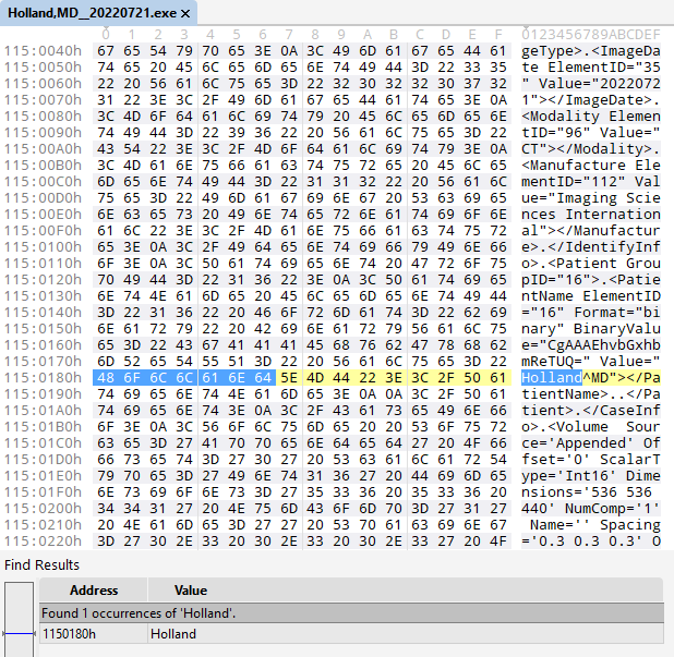
I recognized this as XML data, so I scrolled up until I found what appeared to be the beginning: an opening <INVFile> tag. In XML files, tags come in pairs, so I searched for the accompanying closing tag.
This was all the information I needed to isolate this block into its own file, creatively named invfile.inv. Was that everything I needed? I wasn’t sure yet, so came the next step.
Validating the data
I searched INV file online. On the Anatomage website, it is described as “a proprietary file type. The Invivo file will contain patient’s scan data and work up data in a single file”. I was definitely on the right track.
I eventually came across Invivo Workspace, a web app that can view Invivo case files. I registered an account, uploaded my Invivo case file, and opened it. It worked! I was excited!
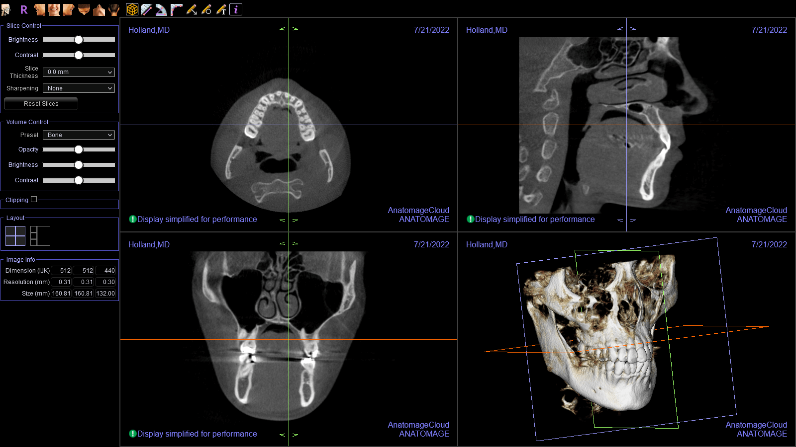
Figuring out the data structure
Now that I confirmed this file contained the data I was interested in, I went to work. The XML portion contained metadata describing the hardware that was used to produce the scan, its creation date, my name: things like that.
More notably, it contained a large binary blob. This, I suspected, is where the CT images live. I isolated it and began looking for patterns.
The most obvious pattern was a recurring watermark which read: Creator: JasPer Version 1.701.0. There happened to be 63 occurrences of this watermark throughout the file. Coincidentally, near the beginning of the file, a 32-bit value equivalent to 63 can be found. Shortly following that is a block of 63 similar values describing the size of each image file. The image files themselves are packed in immediately afterwards.
It’s by way of syllogisms like this, plus some trial and error, that I was able to work out the data structure with no prior knowledge of this file format. It isn’t an exact science, but knowing what design patterns are routinely employed by programmers helps tremendously.
To illustrate this structure to the reader, here’s how it looks if I color-code each section. The pink region stores the number of images, the green region stores the filesize of each image, and the orange region contains the images themselves:
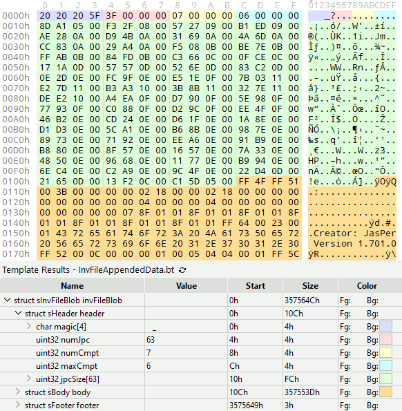
For curious programmers, that’s 010 Editor, a hex editor that supports binary templates. The binary template I wrote for the color coding looks like this:
// Invivo Binary Template
// Holland.vg

// Soft colors
#define cRed    0xddddff
#define cGreen  0xddffdd
#define cBlue   0xffdddd
#define cOrange 0x99ddff
#define cYellow 0xccffff
#define cAqua   0xffffcc

LittleEndian();

struct sInvFileBlob
{
    struct sHeader
    {
        char magic[4] <bgcolor=cBlue>;
        uint32 numJpc <bgcolor=cRed>;
        uint32 numCmpt <bgcolor=cYellow>;
        uint32 lastCmpt <bgcolor=cAqua>;
        uint32 jpcSize[numJpc] <bgcolor=cGreen>;
    } header;

    struct sBody
    {
        local int i;
        local uint32 bg;

        for (i = 0; i < header.numJpc; ++i)
        {
            bg = i & 1 ? cRed : cOrange;

            struct sJpcFile
            {
                byte data[header.jpcSize[i]];
            } jpcFile <bgcolor=bg>;
        }
    } body;

    struct sFooter
    {
        char magic[3] <bgcolor=cBlue>;
    } footer;
} invFileBlob;
Extracting and inspecting an image file
By this point, I had isolated a binary blob from an Invivo case file, which was itself extracted from a Windows executable. Having already worked out the data structure, going one level deeper and extracting an image file was simple enough.
With a little bit of experimentation, I was able to make the following inferences:
-
The image files were created using the JasPer image encoding library.
-
The image files always began with the byte signature
FF 4F FF 51. A quick search revealed this byte signature indicates a JPEG 2000 codestream. Source: List of file signatures - Wikipedia -
Running the file through a JasPer utility named
imginforevealed it is a JPC file specifically, and that it has seven (7) components. -
Each component is a subimage. This means that even though there are 63 image files in the sequence, 63 image files * 7 components each = 441 images in total.
-
The pixel data inside each component is 16-bit LE grayscale.
These findings informed my thinking as I worked towards my goal. I carefully noted them.
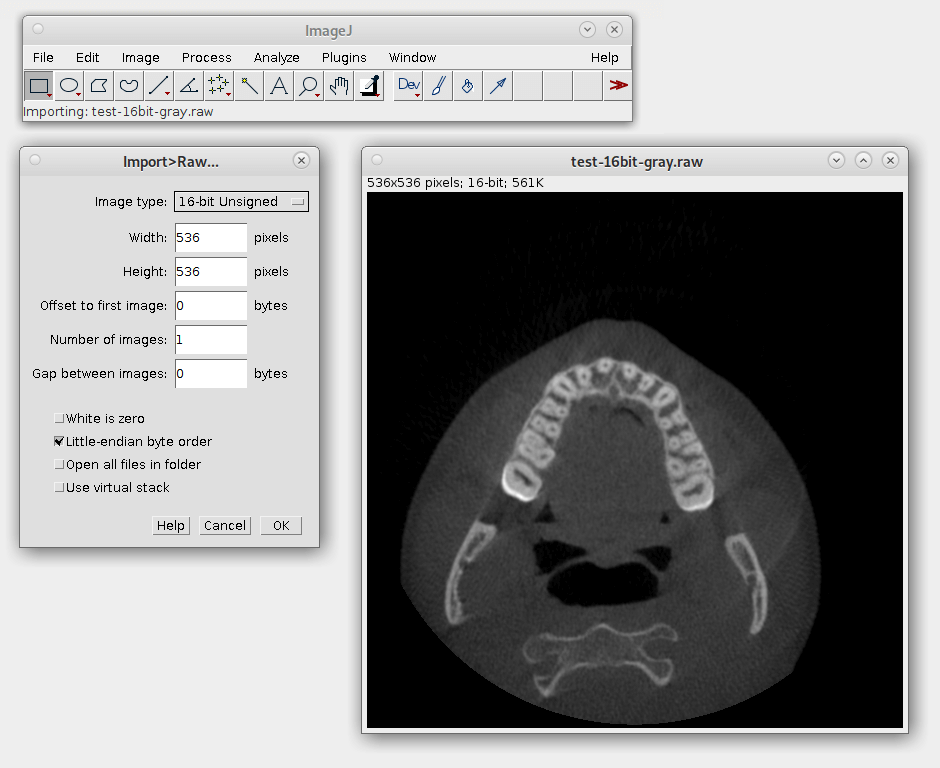
I was able to successfully view one of the images by first converting it to raw pixel data using the following command:
convert test.jpc -depth 16 gray:test-16bit-gray.raw
I then loaded that pixel data into ImageJ, an image processing program developed and maintained by the NIH. It worked!
Displaying CT images using code
In the previous two sections, I worked out the data structure of the binary blob, and I applied my findings to extract and display a single image from it. My next goal was to translate these steps into code the computer could understand.
Here’s what I wanted to do, expressed in pseudo code:
for each image:
   for each channel:
      for each pixel:
         write pixel
It may have been a gross oversimplification of the problem I was trying to solve, but pseudo code doesn’t have to be highly involved. I like to use it as a checklist. If the program can do each of these steps, then it works.
I proceeded to write a program capable of extracting and displaying all the images in rapid succession. This is when things started to get interesting. As you’ll see in the sections that follow, many meaningful things would soon be accomplished using this data.
CT “video” displayed by my program.
Adding color
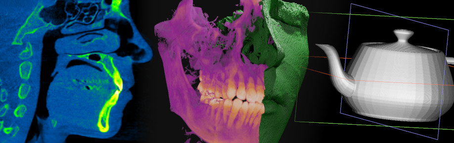
Grayscale is the simplest possible visual representation of a scan: the density of a given point is interpreted as a brightness value. Denser materials such as bone and amalgam come across more brightly than softer tissues and empty passageways.
Color palettes are regularly used when interpreting medical images because they can highlight details that might otherwise go unnoticed, so I sought to include them in my program.
Implementation of this key feature was simple: instead of treating the density as brightness, it is mapped to a point on a predefined color spectrum.
Deriving the other anatomical planes
A CT scan is a sequence of two-dimensional images, but what would happen if you were to theoretically print all of those images onto individual pieces of paper, stack them up, and cut the stack into two halves, allowing you to peer inside? A third dimension would be revealed! This is the 3D nature of CT scans. By doing this via code, we can see the other anatomical planes.
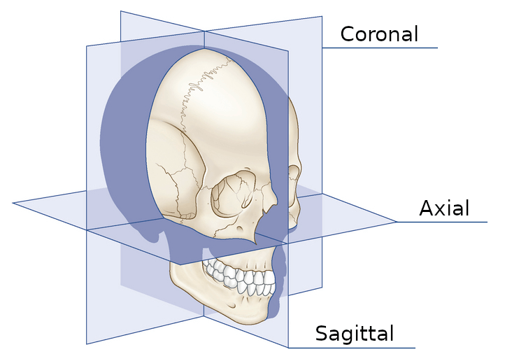
If, in a given image, the X and Y axes represent points existing within the axial plane, then the Z axis refers to other images directly before or after it in the sequence. With this in mind, X, Y, and Z can be cleverly shuffled to produce images of the other planes.

The axial, sagittal, and coronal anatomical planes, respectively, displayed by my program.
The moving axis line illustrates the relation between the axial and sagittal planes.
Generating point clouds
In the last section, we established that each pixel in each image represents a point in 2D space, and that if all images are accounted for, each pixel actually represents a point in 3D space. We can use this information to construct a 3D point cloud. And because I already programmed color palettes, the point clouds can be just as vivid and colorful as the images themselves!
The following results were exported from my software and rendered in Blender.
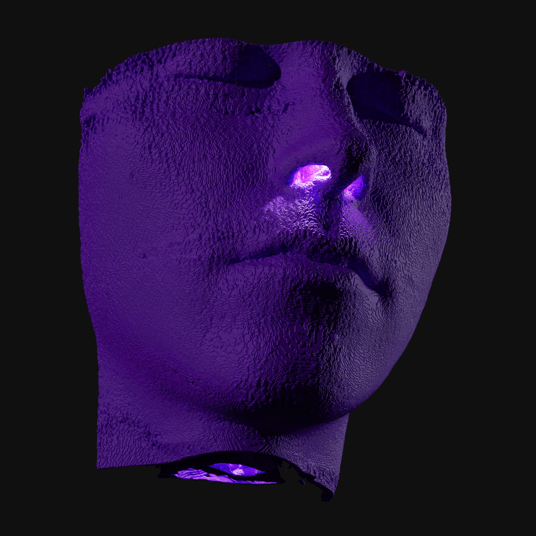
My dental CBCT scan, interpreted as a 3D point cloud. I recognize that face!
When I was still in the exploratory phase, I wanted to work with a simplified data set, so I implemented a basic point density algorithm. Pictured: Point clouds of varying densities, overlaid. Higher point densities reveal more detail.
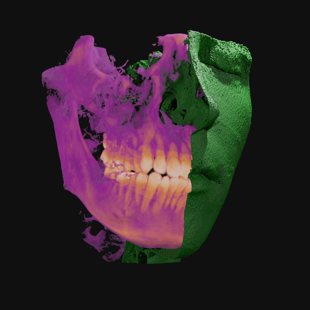
Point clouds can be manipulated in many ways. Here, I wrote code to isolate the outermost layer of soft tissue from bone before cutting away half.
Reversing the entire process
What if I wanted to create my own Invivo case file? I don’t have a CBCT machine, but I can still simulate a scan! All I need is a 3D model and a way to cut it into slices. I decided to make my first test subject the famous Utah Teapot.
In Blender, I set up an orthographic camera pointing down towards the teapot. Next, I added a geometric plane that moves through the teapot from top to bottom. This plane has a boolean operator attached to it. The boolean operator discards any geometry that doesn’t happen to intersect with the teapot.
That’s a lot to take in, so I rendered the following animation to illustrate:

Then I added two new features to my program. It needed to be able to:
-
Import image sequences.
-
Export Invivo case files.
Once I got that working, I opened the resulting file in Invivo Workspace. I was quite happy with how it turned out!
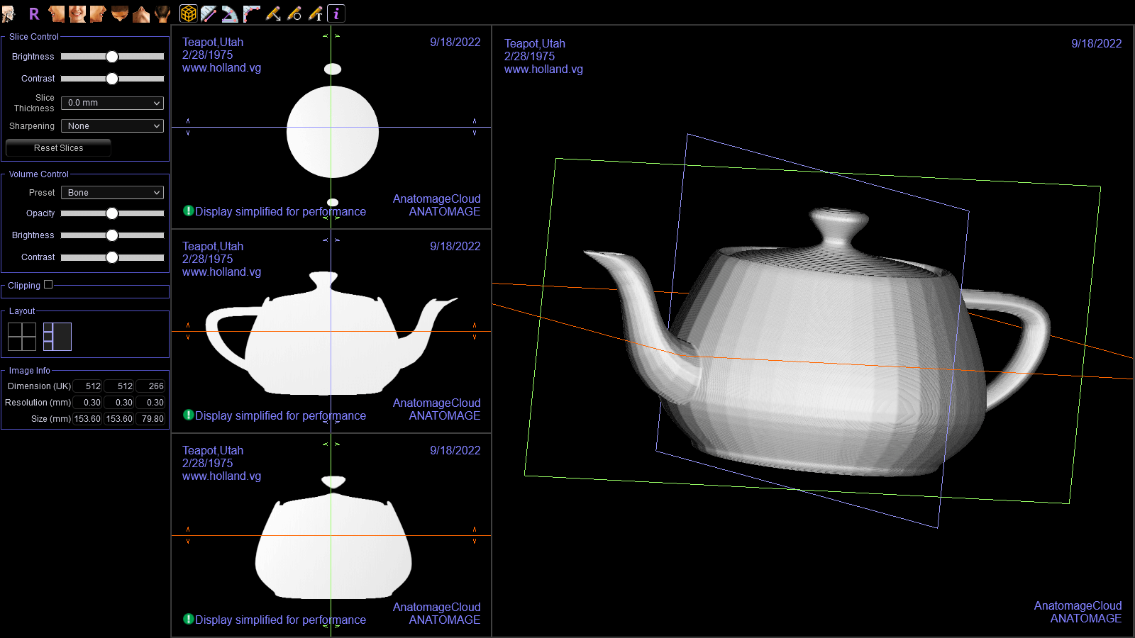
Check out the watermark I added!
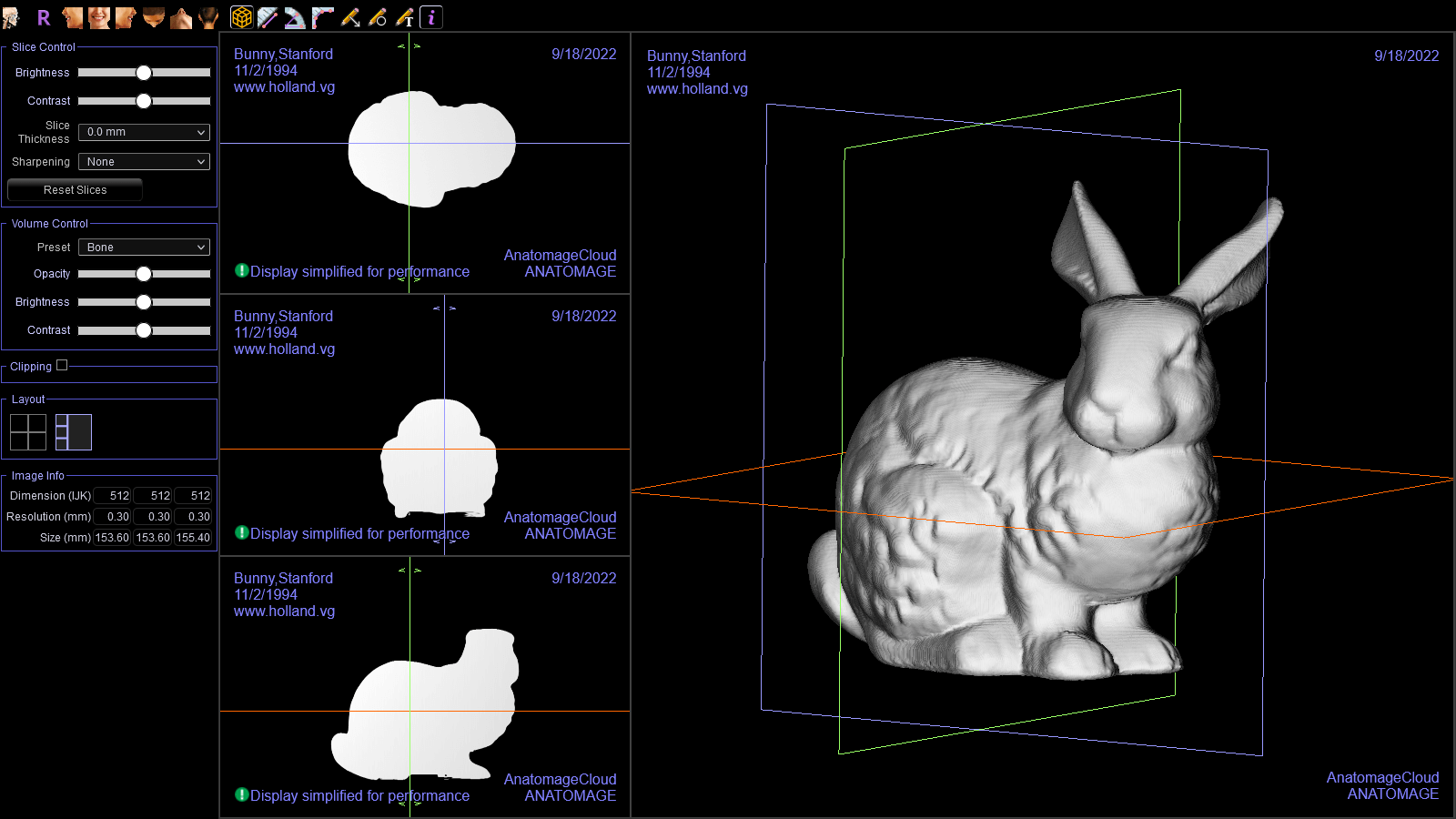
I performed the same test with the Stanford Bunny.
And then I prepared a more complex model. I wanted something with both bone and soft tissue so the final test could be more realistic.
This simulated CT scan of a cow is the culmination of my work.
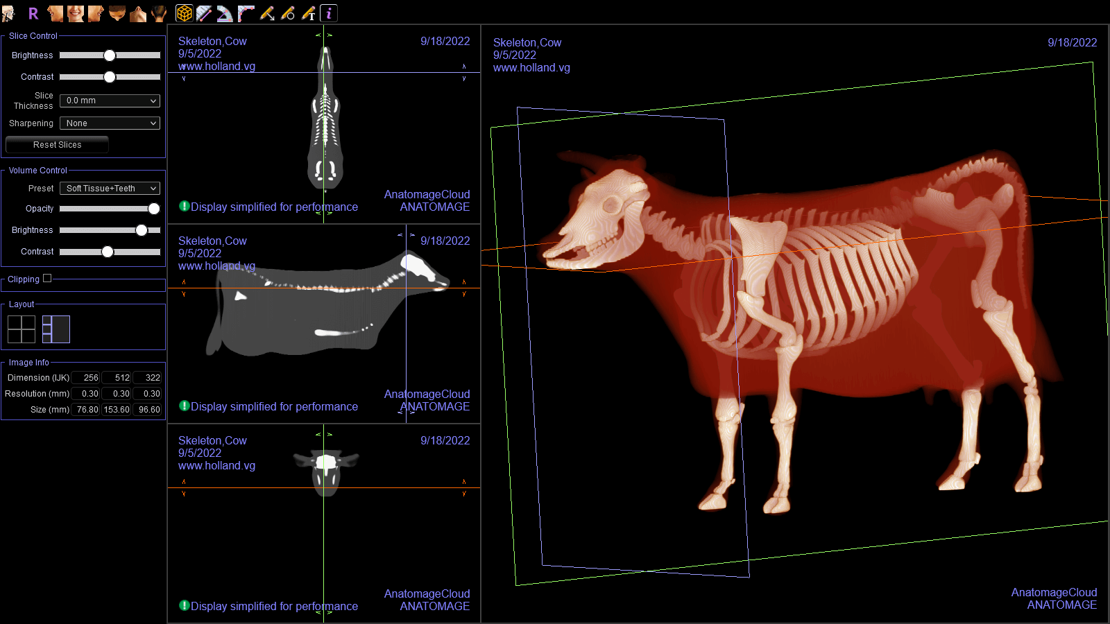
And here it is displayed in Invivo Workspace.
In closing
For a long time, I’ve been wanting to work with medical imaging data, and this was the perfect opportunity. I worked on this for a few weekends and I had a lot of fun.
For extra curious readers wanting to conduct their own experiments, all relevant files and the full source code for this project can be found on GitHub: z64me/invivo-cbct
Attribution
The following software libraries made this project possible: